Cyclistic Case Study

In today’s data-driven world, the ability to analyze and interpret data is crucial for making informed decisions. As part of the Data Analytics Certificate program, this capstone project focuses on the Cyclistic bike-sharing dataset, which provides a rich source of information on bike usage patterns in a major metropolitan area. By leveraging this dataset, I aim to uncover insights into user behavior, identify trends, and provide actionable recommendations to enhance the bike-sharing experience. This project not only demonstrates the practical application of data analytics skills but also contributes to the growing field of sustainable urban transportation.

About the Company

In 2016, Cyclistic launched a successful bike-share offering. Since then, the program has grown to a fleet of 5,824 bicycles that are geo-tracked and locked into a network of 692 stations across Chicago. The bikes can be unlocked from one station and return to any other station in the system anytime. Until now, Cyclistic’s marketing strategy relied on building general awareness and appealing to broad consumer segments. One approach that helped make these things possible was the flexibility of its pricing plans: single-ride passes, full-day passes, and annual memberships.

Customers who purchase single-ride or full-day passes are referred to as casual riders. Customers who purchase annual memberships are Cyclistic members. Cyclistic’s finance analysts have concluded that annual members are much more profitable than casual riders. Although the pricing flexibility helps Cyclistic attract more customers, Moreno believes that maximizing the number of annual members will be key to future growth. Rather than creating a marketing campaign that targets all new customers, Moreno believes there is a very good chance to convert casual riders into members. She notes that casual riders are already aware of the Cyclistic program and have chosen Cyclistic for their mobility needs.

Moreno has set a clear goal: Design marketing strategies aimed at converting casual riders into annual members. To do that, however, the marketing analyst team needs to better understand how annual members and casual riders differ, why casual riders would buy a membership, and how digital media could affect their marketing tactics. Moreno and her team are interested in analyzing the Cyclistic historical bike trip data to identify trends.

Define the Problem

The main problem for the director of marketing and marketing analytics team is this: Design marketing strategies aimed at converting Cyclistic’s casual riders into annual members. There are three questions that will guide this future marketing program. For the scope of this project, I will answer the following questions:

• How do annual members and casual riders use Cyclistic bikes differently?
• Why would casual riders buy Cyclistic annual memberships?
• How can Cyclistic use digital media to influence casual riders to become members?

By analyzing the data, we can identify broad patterns within the two groups. Understanding these differences will enable us to create more accurate customer profiles for each group. These insights will assist the marketing analytics team in designing high-quality, targeted marketing strategies to convert casual riders into members. For the Cyclistic executive team, these insights will help maximize the number of annual members and drive future growth for the company.

The Task

Analyze historical bike trip data to identify trends in how annual members and casual riders use Cyclistic bikes differently and create a data-driven digital media campaign to increase ridership.

Environment Setup

• readr for loading CSV files
• scales for better graph scales
• tidyverse and dplyr for knitting file
• conflicted to manage and set conflict repairs
• ggplot2 for visuals
• fontawesome & paletteer for a pretty notebook

Load Data from CSV

q1_2019 <- read_csv("CSV/Divvy_Trips_2019_Q1.csv")
q1_2020 <- read_csv("CSV/Divvy_Trips_2020_Q1.csv")

Clean and Combine

Verify Column Names

colnames(q1_2019)
colnames(q1_2020)

Rename Columns of ‘q1_2019.csv’ for Consistency

q1_2019 <- rename(q1_2019
 ,ride_id = trip_id
 ,rideable_type = bikeid
 ,started_at = start_time
 ,ended_at = end_time
 ,start_station_name = from_station_name
 ,start_station_id = from_station_id
 ,end_station_name = to_station_name
 ,end_station_id = to_station_id
 ,member_casual = usertype
 )

Inspect the Dataframes

str(q1_2019)
str(q1_2020)

Convert ride_id and rideable_type columns to CHR

q1_2019 <- mutate(q1_2019, ride_id = as.character(ride_id), rideable_type = as.character(rideable_type))

str(q1_2019)

Create and Clean New Table ‘all_trips’

Stack Quarter Dataframes into One

all_trips <- bind_rows(q1_2019, q1_2020)

Remove lat, long

all_trips <- all_trips %>%
  select(-c(start_lat, start_lng, end_lat, end_lng, tripduration))

Load ‘all_trips’ and Preview

#colnames(all_trips)
#nrow(all_trips)
#dim(all_trips)
#head(all_trips)
#str(all_trips)
summary(all_trips) #only one line needed

Clean ‘member_casual’ Column for Consistency

#table(all_trips$member_casual) #view table for memberships
all_trips <- all_trips %>%
  mutate(member_casual = recode(member_casual ,"Subscriber" = "member" ,"Customer" = "casual"))
table(all_trips$member_casual) #verify table update contains 2 variables

Split Date into Columns for Better Aggregation

all_trips$date <- as.Date(all_trips$started_at) #The default format is yyyy-mm-dd
all_trips$month <- format(as.Date(all_trips$date), "%m")
all_trips$day <- format(as.Date(all_trips$date), "%d")
all_trips$year <- format(as.Date(all_trips$date), "%Y")
all_trips$day_of_week <- format(as.Date(all_trips$date), "%A")

Add ‘ride_length’ Calculation and Make Numeric

all_trips$ride_length <- difftime(all_trips$ended_at,all_trips$started_at)
#is.factor(all_trips$ride_length)
all_trips$ride_length <- as.numeric(as.character(all_trips$ride_length))
is.numeric(all_trips$ride_length) #verify numeric

Remove the Rows of Bad Data

data frame include a few hundred entries when bikes were removed for service

all_trips_v2 <- all_trips[!(all_trips$start_station_name == "HQ QR" | all_trips$ride_length<0),]

Prepare Descriptive Analysis

Analyze Ride Lengths

#calculate all ride lengths
#mean(all_trips_v2$ride_length) #average (total ride length / rides)
#median(all_trips_v2$ride_length) #midpoint ride length
#max(all_trips_v2$ride_length) #longest ride
#min(all_trips_v2$ride_length) #shortest ride
# or more simply on one line
summary(all_trips_v2$ride_length)

Compare Casual and Members

aggregate(all_trips_v2$ride_length ~ all_trips_v2$member_casual, FUN = mean)
aggregate(all_trips_v2$ride_length ~ all_trips_v2$member_casual, FUN = median)
aggregate(all_trips_v2$ride_length ~ all_trips_v2$member_casual, FUN = max)
aggregate(all_trips_v2$ride_length ~ all_trips_v2$member_casual, FUN = min)

Correct Day of Week Order

all_trips_v2$day_of_week <- ordered(all_trips_v2$day_of_week, levels=c("Sunday", "Monday", "Tuesday", "Wednesday", "Thursday", "Friday", "Saturday"))
aggregate(all_trips_v2$ride_length ~ all_trips_v2$member_casual + all_trips_v2$day_of_week, FUN =mean)

Analyze Data by Type and Weekday

all_trips_v2 %>%
  mutate(weekday = wday(started_at, label = TRUE)) %>% #creates weekday field using wday
    group_by(member_casual, weekday) %>% #groups by usertype and weekday
      summarise(number_of_rides = n(), average_duration = mean(ride_length)) %>%
        arrange(member_casual, weekday)

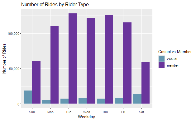
Visualize Number of Rides by Rider Type

all_trips_v2 %>%
  mutate(weekday = wday(started_at, label = TRUE)) %>%
    group_by(member_casual, weekday) %>%
      summarise(number_of_rides = n(), average_duration = mean(ride_length)) %>%
        arrange(member_casual, weekday) %>%
          ggplot(aes(x = weekday, y = number_of_rides, fill = member_casual)) +
          geom_col(position = "dodge") +
          scale_x_discrete(name="Weekday") +
          scale_y_continuous(labels=comma, name="Number of Rides") +
          labs(title = "Number of Rides by Rider Type", fill= "Casual vs Member") +
          scale_fill_paletteer_d("PrettyCols::Bold")

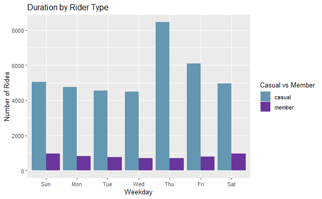
Visualize Average Duration by Rider Type

all_trips_v2 %>%
  mutate(weekday = wday(started_at, label = TRUE)) %>%
    group_by(member_casual, weekday) %>%
      summarise(number_of_rides = n(), average_duration = mean(ride_length)) %>%
        arrange(member_casual, weekday) %>%
          ggplot(aes(x = weekday, y = average_duration, fill = member_casual)) +
          geom_col(position = "dodge") +
          scale_x_discrete(name="Weekday") +
          scale_y_continuous(name="Number of Rides") +
          labs(title = "Duration by Rider Type", fill= "Casual vs Member") +
          scale_fill_paletteer_d("PrettyCols::Bold")

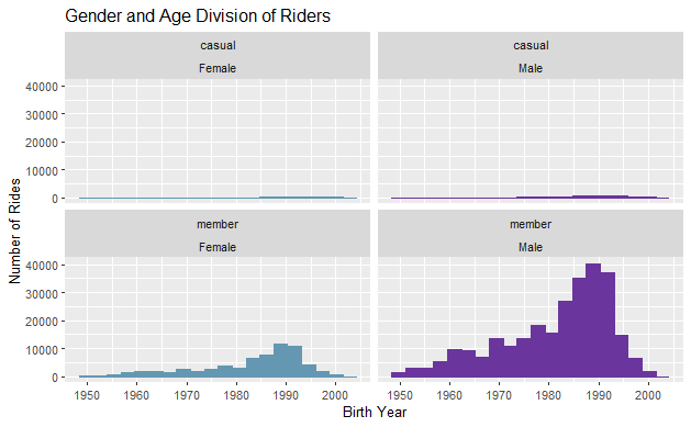
Visualise Gender and Age Division of Riders

all_trips_v2 %>%
  filter(!is.na(gender)) %>%
  filter(birthyear >= 1950L & birthyear <= 2003L & !is.na(birthyear)) %>%
  ggplot() +
  aes(x = birthyear, color = gender, fill = gender) +
  geom_histogram(bins = 20L, show.legend = FALSE) +
  facet_wrap(vars(member_casual, gender)) +
  scale_x_continuous(name="Birth Year") +
  scale_y_continuous(name="Number of Rides") +
  labs(title = "Gender and Age Division of Riders") +
  scale_fill_paletteer_d("PrettyCols::Bold") +
  scale_color_paletteer_d("PrettyCols::Bold")

Export Summary File for Further Analysis

counts <- aggregate(all_trips_v2$ride_length ~ all_trips_v2$member_casual +
                      all_trips_v2$day_of_week, FUN = mean,)
write.csv(counts, file = 'output_CSV/avg_ride_length.csv')

Observations

• Casual users have significantly longer rides on Sundays compared to members.
  
• Casual users have much shorter rides on weekdays compared to members.
  
• Casual users typically have longer ride lengths than members.
  

Recommendations

• Create weekend specific memberships plans, the “Weekend Warrior” plan.
  
• Highlight benefits for daily commuters, the “Bike 2 Work” plan.
  
• Implement a tiered membership to reward longer rides.
  
• Create loyalty program with points, redeemed for merch from local partners.
  

Find this Project on the Web!

Kaggle Notebook in Python
Kaggle Notebook in R
Tableau Dashboard